Using BERT for topic modeling (Python)

What are the main topics of a text, or of a set of texts?

Sometimes in marketing — but also in the humanities, such as literature, history, sociology — you need to analyse a large corpus made of many documents. One thing you want to investigate is: “what are these texts about?” and another is “can we classify these texts by their prevailing topic?”.

A marketing example might be:

Given a set of conversations about a certain brand, what are the prevailing topics? How much do they weigh on the total?

Approach #1: the LDA model

The most common technique is Latent Dirichlet Allocation, introduced by Blei, Ng and Jordan in 2002. It’s versatile: it ignores language and its structures and relies on the bag-of-words model. In simple terms: a matrix is built with all the individual words as columns and the documents as rows; the values are the number of occurrences of each word in each document.

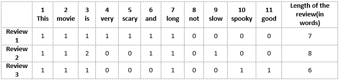
esempio di una Bag of Word con tre documenti (recensioni in questo caso)

The problems

1. Removal of meaningless words is done quite crudely: words above a certain frequency are dropped, plus an a-priori list of “stopwords”. If this cleaning is poor, the topics are hard to interpret.
2. The model relies on a pre-set number of topics. It works well on a narrow corpus, but on larger corpora you may need to identify 20, 30, 40 topics.
3. The model forces every document into a topic. It assigns each document a probability of belonging to a topic (summing to 100). There will always be a most-probable topic, even if the document is about none of them.

How to solve this? By using the best of Google’s AI: BERT.

Approach #2: BERT combined with c-TF-IDF

I’m writing this because there’s a gap among Italian blogs on how to do topic modeling with BERT. It’s largely based on this article by Maarten Grootendorst, creator of BERTopic.

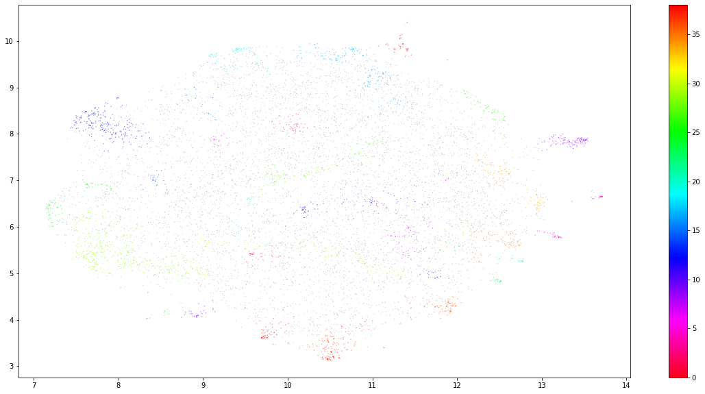
Output dell’analisi. I colori identificano alcuni topic individuati

1. Dataset + libraries

The starting dataset is a database of more than 12,000 songs labelled “indie” and “non-indie”, released between 2000 and 2020, including lyrics and some Spotify metrics. Importantly, the lyrics are all lowercase and without punctuation.

import pandas as pd
from sentence_transformers import SentenceTransformer  # NB: you may need pyTorch installed
import umap        # needed for dimensionality reduction
import hdbscan     # needed for clustering
import matplotlib.pyplot as plt
import numpy as np
from sklearn.feature_extraction.text import CountVectorizer

Then we load the dataset:

path = 'C:/Users/User/Downloads/'
filename = 'INDIE DATABASE.csv'
data_raw = pd.read_csv(path + filename)

# keep only songs labelled as indie
data_indie = data_raw[data_raw['label'] == 'indie']

# build a list with all the lyrics
data = list(data_indie['TESTO'])

2. Creating the embeddings

The first step is converting the documents into numerical data. We use BERT, which extracts context-based groupings (embeddings) from a text. There are many pre-trained models available. We’ll use the sentence_transformers library, whose embeddings work well at the single-document level.

model = SentenceTransformer('distilbert-multilingual-nli-stsb-quora-ranking')
embeddings = model.encode(data, show_progress_bar=True)

Note: we use DistilBERT, a multilingual pre-trained model with a good speed/performance trade-off. Our documents are now 768-dimensional vectors.

NOTE: very large documents may cause errors. Try splitting them into single paragraphs.

3. Clustering

We want documents about the same subjects to cluster together. First, though, we must reduce the dimensionality of the embeddings, since many clustering algorithms struggle with high dimensions.

Part I — UMAP. We reduce dimensionality with UMAP, which preserves local structure well even at lower dimensions. We reduce to 5 dimensions, keeping the local neighborhood at 15.

umap_embeddings = umap.UMAP(n_neighbors=15,
                            n_components=5,
                            metric='cosine').fit_transform(embeddings)

Part II — HDBSCAN. A density-based algorithm that pairs well with UMAP and treats unassigned points as outliers rather than forcing them into a cluster.

cluster = hdbscan.HDBSCAN(min_cluster_size=15,
                          metric='euclidean',
                          cluster_selection_method='eom').fit(umap_embeddings)

4. Data visualization

Using matplotlib:

# Prepare data
umap_data = umap.UMAP(n_neighbors=15, n_components=2, min_dist=0.0, metric='cosine').fit_transform(embeddings)
result = pd.DataFrame(umap_data, columns=['x', 'y'])
result['labels'] = cluster.labels_

# Visualize clusters
fig, ax = plt.subplots(figsize=(20, 10))
outliers = result.loc[result.labels == -1, :]
clustered = result.loc[result.labels != -1, :]
plt.scatter(outliers.x, outliers.y, color='#BDBDBD', s=0.05)
plt.scatter(clustered.x, clustered.y, c=clustered.labels, s=0.05, cmap='hsv_r')
plt.colorbar()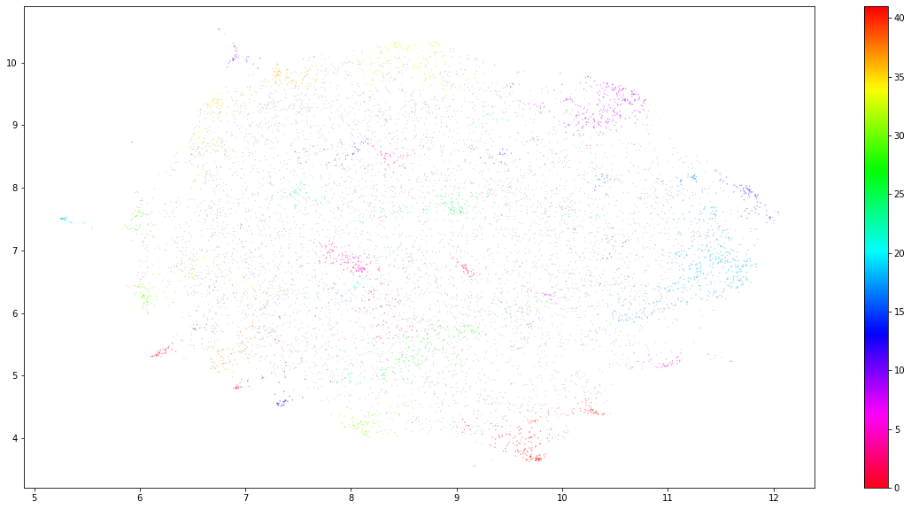

5. Creating the topics

First, a document-topic dataframe:

docs_df = pd.DataFrame(data, columns=["Doc"])
docs_df['Topic'] = cluster.labels_
docs_df['Doc_ID'] = range(len(docs_df))

But what are these topics? We apply TF-IDF not to a single document, but to all documents sharing a topic. This variant, c-TF-IDF (‘c-’ for class-based), treats all documents of a topic as one big document, so the score reflects the most important words of the whole topic.

# merge documents that share the same topic
docs_per_topic = docs_df.groupby(['Topic'], as_index=False).agg({'Doc': ' '.join})

# define the c_tf_idf function
def c_tf_idf(documents, m, ngram_range=(1, 1)):
    count = CountVectorizer(ngram_range=ngram_range, stop_words="english").fit(documents)
    t = count.transform(documents).toarray()
    w = t.sum(axis=1)
    tf = np.divide(t.T, w)
    sum_t = t.sum(axis=0)
    idf = np.log(np.divide(m, sum_t)).reshape(-1, 1)
    tf_idf = np.multiply(tf, idf)
    return tf_idf, count

tf_idf, count = c_tf_idf(docs_per_topic.Doc.values, m=len(data))

6. Interpreting the topics

Take the top 20 words per topic by c-TF-IDF score:

def extract_top_n_words_per_topic(tf_idf, count, docs_per_topic, n=20):
    words = count.get_feature_names()
    labels = list(docs_per_topic.Topic)
    tf_idf_transposed = tf_idf.T
    indices = tf_idf_transposed.argsort()[:, -n:]
    top_n_words = {label: [(words[j], tf_idf_transposed[i][j]) for j in indices[i]][::-1] for i, label in enumerate(labels)}
    return top_n_words

def extract_topic_sizes(df):
    topic_sizes = (df.groupby(['Topic'])
                     .Doc
                     .count()
                     .reset_index()
                     .rename({"Topic": "Topic", "Doc": "Size"}, axis='columns')
                     .sort_values("Size", ascending=False))
    return topic_sizes

top_n_words = extract_top_n_words_per_topic(tf_idf, count, docs_per_topic, n=20)
topic_sizes = extract_topic_sizes(docs_df); topic_sizes.head(15)

With topic_sizes you see how frequent each topic is. Note: documents labelled -1 were not assigned to any topic. Good or bad? It depends on your research intent.

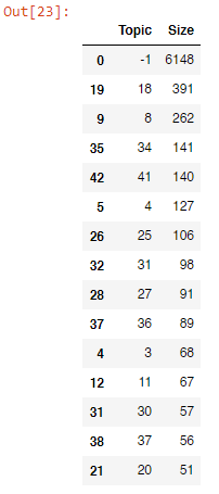
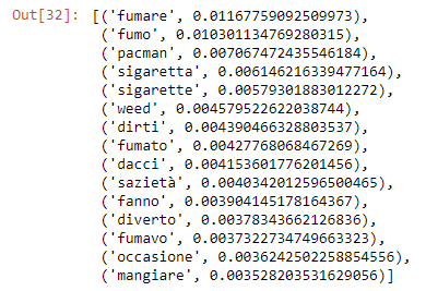
To explore a topic’s content, just run top_n_words[4][:15] to see the 15 most important words of topic 4. Enjoy!

NOTE: all the code is here: BERTopic on GitHub.